Class 4. Boltzmann machine
Constructing an Autoencoder model looks like an art, if not computationally heavy work. A lot of non-trained data engineers rely on coding libraries and a graphics card (that supports ‘AI’ computation), and hoping the computer to find an ideal Neural Network. As discussed in previous section, the process is highly exposed to overfitting, local maxima, and humongous computational cost. There must be more elegant, more reasonable, and more scientific way to do so.
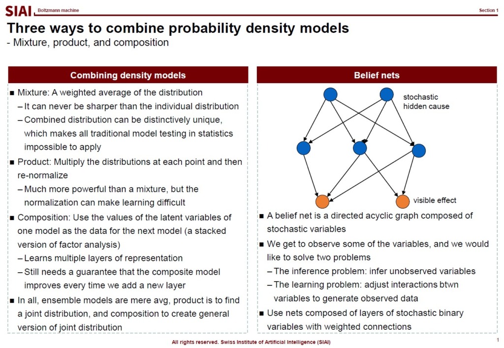
Let’s think about a multi-layered neural network model. From the eyes of Factor Analysis, each layer is one round of factor analysis. The factor analysis is in fact a re-contruction of vector space, as was discussed in PCA. In sum, the multi-layered neural network model is a series of re-constructions in vector space. What is the re-construction doing? By PCA, it orthogonalizes data’s dimension. Factor analysis in general changes the vector space’s key axes. In statistical terms, it is a transformation of density functions from one to another. Both processes preserve the data’s hidden information. The vector space as a whole is the same. Only axes are different. Density functions are different, but information in the data set is still the same.

Since each node is a marginal density function and the combination of them on each layer is a joint density, moving from one layer to another layer is a transformation of one joint density to another. In the density, it is no more than a multiplication of functions, if they are independent. However, between two layers, we know that the deep learning structure has dependency to each other. Assuming that the first layer is the data input, then the second layer depends on how much weights are assigned to each link. Depending on the structure of the second layer and weights, the third layer is affected. Once the feed forward process is done, then the back propagation is the opposite process. Though the chain rule helps us to avoid painstaking calculations in each step, nonetheless, the dependency to each layer remains.
This is where we need MCMC, or more specifically Gibbs sampling type approximation. Note that Gibbs sampling assumes input data’s distribution, and expects what will be the outcome’s density. Once done, then the outcome’s density becomes the new input, and we use the information to re-construct the outcome, which is the original input. By running back and forth, the process is expected to converge. Although the correlation between nodes can be a bothersome issue, either over- or under-estimating key weights, such irregularity can be handled by Metropolis-Hastings type corrections. Gibbs class samplings are, in short, two groups of dependent sampling process, instead of a single group. The Bayesian technique precisely fits to our autoencoder problem.

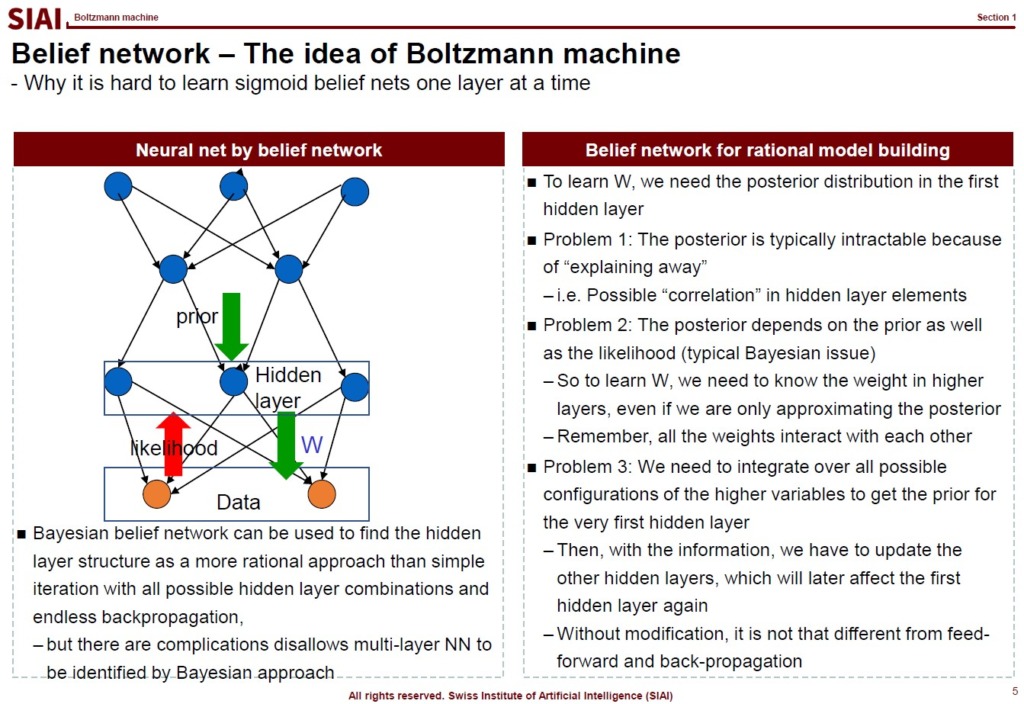
Note that constructing a belief network for rational model has to deal with multiple intrinsic problems. (Mentioned in the aboved screen-captured lecture note). All of them can be successfuly handled by Gibbs type autoencoder.
The structure is known as ‘Restricted Boltzmann Machine (RBM)’.

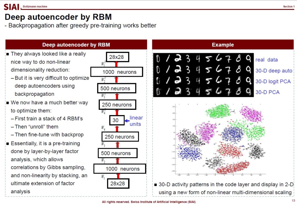
As is illustrated in the above lecture note, the model can capture key hidden factor components better than PCA.


