Class 5. Image recognition
As shown by RBM’s autoencoder versions, if the neural network is well-designed, it can perform better than PCA in general when it comes to finding hidden factors. This is where image recognition relies on neural network.
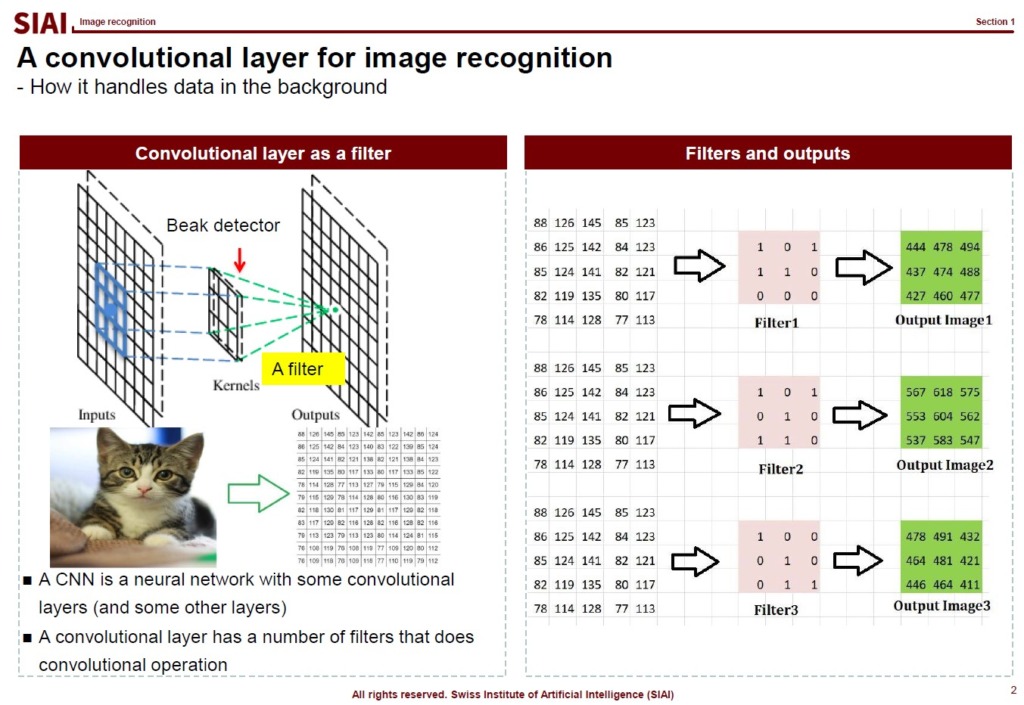
Images are first converted to a matrix with RGB color value, (R, G, B), entries. The matrix is for the coordination of each RGB color value. If three dimensional image, then you need a tensor with RGB color value entries. In below sample, I took the average value of RGB entries for better understanding. In fact, if it is black/white, you only need the matrix, because (R, G, B) can be translated to a single 0~1 value.

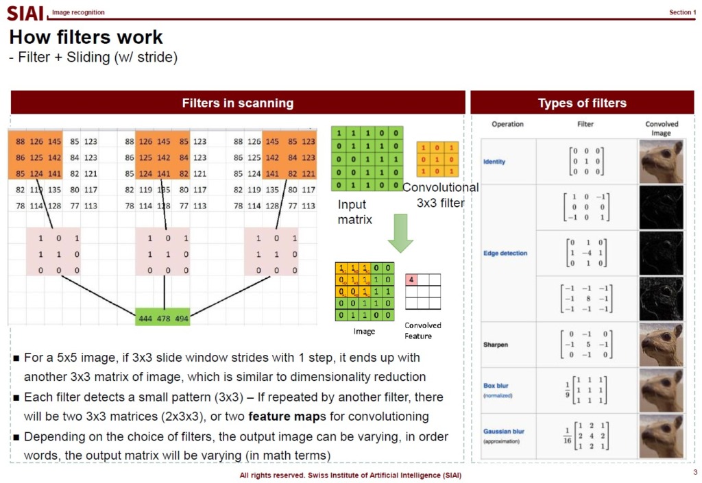
When a modeler tries to feed the image data to the model, it relies on sliding for various reasons. The slider is also known as a filter, which is widely used for photo filtering. SNS images, for example, are frequently modified. The filter you can find in the photo app or an SNS app is basically the same as the slider that we use in image recognition.

Depending on your choice of the filter, the output matrix becomes different. It may help you to have black/white effect or sharpening. There are thousands of different filters.
One of the key reasons that we rely on the slider in image recognition is, after the sliding, the feed data size becomes smaller. The higher resolution the image is, the more data the Neural Network has to process. Given that Neural Network model is known as one of the the most computational cost consuming method, it is strictly preferred to reduce the image data size. One does not want to lose the important features of the data, just like we use PCA. This is why the choice of filter is a key component of the successful image recognition. For some images, filter A can perform magnificently better than filter B.

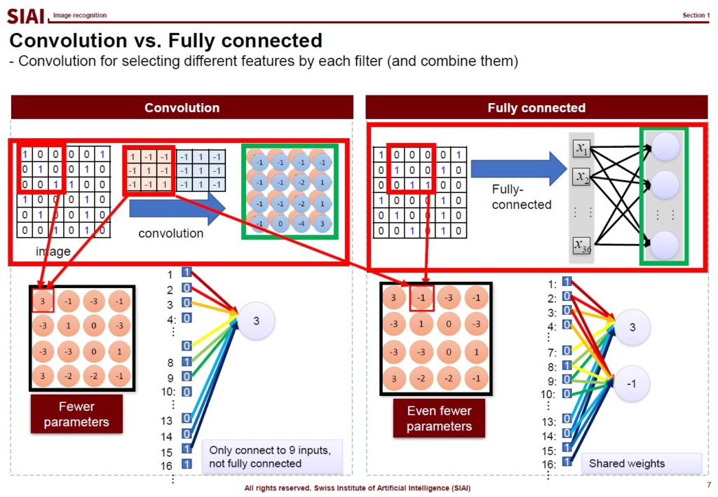
Another technique that we rely on for image recognition is convolutioning. From the slided, or scanned, image data, fully connected neural network forces us to find weights for all links. The convolution helps us to avoid such overlaps, which can further minimize computational costs.

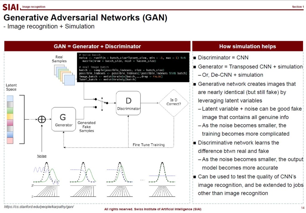
To help you to understand that CNN based image recognition model is still an extension of factor analysis, let’s talk little bit of Generative Adversarial Networks (GAN).
The model captures a couple of latent features of the image at the beginning. Just like the first stage of autoencoder, the choise of latent nodes is a key to build a winning model in accuracy and speed. From the latent components, the CNN’s convolutioning helps us to further speed up finding weights. The GAN model itself is just another variation of MCMC sampling. You just create a lot of images with some random error from the same latent space. The error imposed images are considered fake images. Your discreminator is supposed to exclude the fakes. It then becomes a simple classification problem. By the artificially created fake image data, the model can learn from more number of data. As discussed in COM501: Scientific Programming, the simulation can help us to find the true population in that $I_M \rightarrow I$ as $M \rightarrow \infty$.


