Class 2. Autoencoder

Feed forward and back propagation have significant advantage in terms of speed of calculation and error correction, but it does not mean that we can eliminate the errors. In fact the error enlarges if the fed data leads the model to out of convergence path. The more layers there are, the more computational resources required, and the more prone to error mis-correction due to the structure of serial correction stages in every layer.

The reason we rely on Neural Network model is because we need to find a nested non-linear structure of the data set, which cannot be done by other computational models, such as SVM. Then, is there a way to fix the mis-correction? Partly, it can be done by drop-outs, but one has to compromise loss of information and the structure of drop-out is also arbitrary.

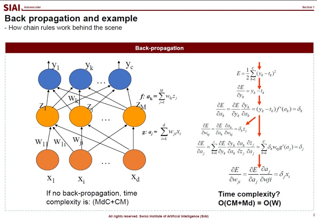
What, instead, can be done is to build an autoencoder model in a way to replicate Factor Analysis in network form. Recall from Machine Learning that Factor Analysis is a general form of Principle Component Analysis (PCA). Though PCA is only limited to linear combination of variables to re-construct the data’s vector spaces by variance-covariance matrix. Given that all computational models are in a way to re-structure original data sets to our desired form, PCA could help us to find hidden key components of variance’s dimension. i.e. the target of all regression based models, including Neural Network, is to maximize explanatory power in terms of variability matching.

From the vector space of second moments, the combination of explanatory variables does not necessarily have to be linear. This is why we moved away from linear regression and have been exploring all non-linear models. The same works for hidden factors. The combination of variables to match hidden factors does not, again, have to be linear. In Factor Analysis, we have explored a bit that depending on the data’s underlying distribution, factor combination can be non-linear.

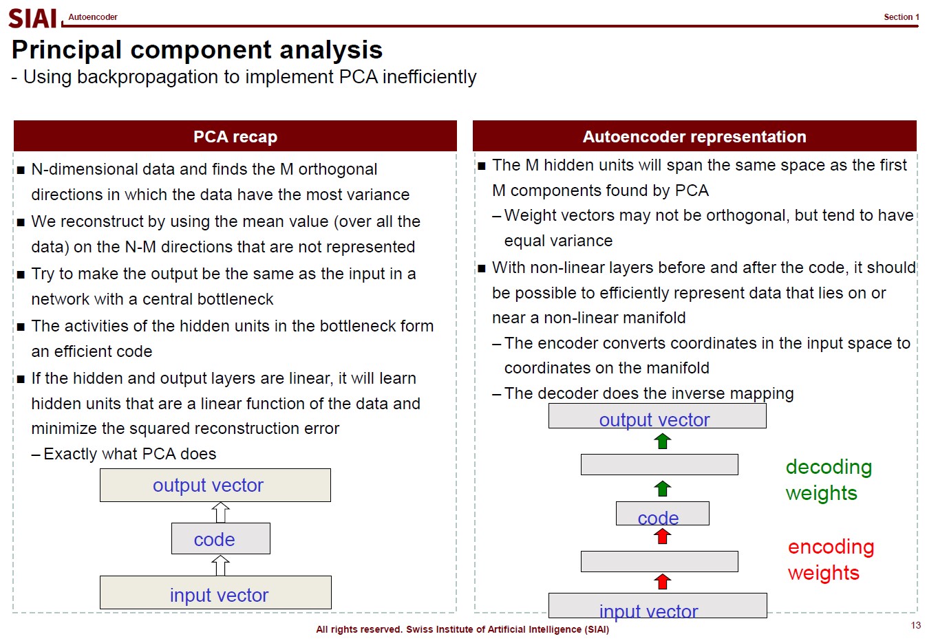
Here comes the benefit of Autoencoder. We can construct Neural Network model with the concept of Factor Analysis. With the right number of hidden factors, the re-designed Neural Network model not only becomes more robust to changes in data sets, but it also becomes less prone to error mis-correction and/or over-fitting. If one have more than needed hidden factors, it is likely the model is going to be overfit. To deal with it, most frequent choice is drop-out, but the result, as mentioned earlier, is not robust, and sometimes it is no more than an improvision for that specific learning event. To small number of hidden factors in a particular layer obviously results in insufficient learning.

To help you to follow Autoencoder’s logic in network building, let’s talk about matching number 0 to 9 in shapes in image recognition. By PCA, as discussed in Machine Learning, one tries to find PCs from transformed image. Some PCs may help us to differenciate 0 and 3, but that particular PC is not the strongest vector space that we usualy look for in PCA based regressions (PCR). Together with other similar images like 9, the upper right parts of the images will give us one PC due to commonality. Here in image recognition, we need PCs from common parts for some guessing, at the same time we also need uncommon parts’ PC to differentiate 0, 3, and 9. There could be over 100 PCs initially, but eventually, we need 10 hidden factors to verify 0 to 9.

The same thought experiment can be constructed by a rather a huge size of Neural Network. Your end layer will have 10 nodes, but at the beginning, you may need over 100 nodes, just like PCA. The construction of multiple hidden layers in the middle, coined as ‘Encoder’, should be carefully designed to pick up separable PCs at first, then exclude unnecessary PCs for the end goal. Like we have witnessed in tree-based models, creating a non-linear function requires a number of different layers.

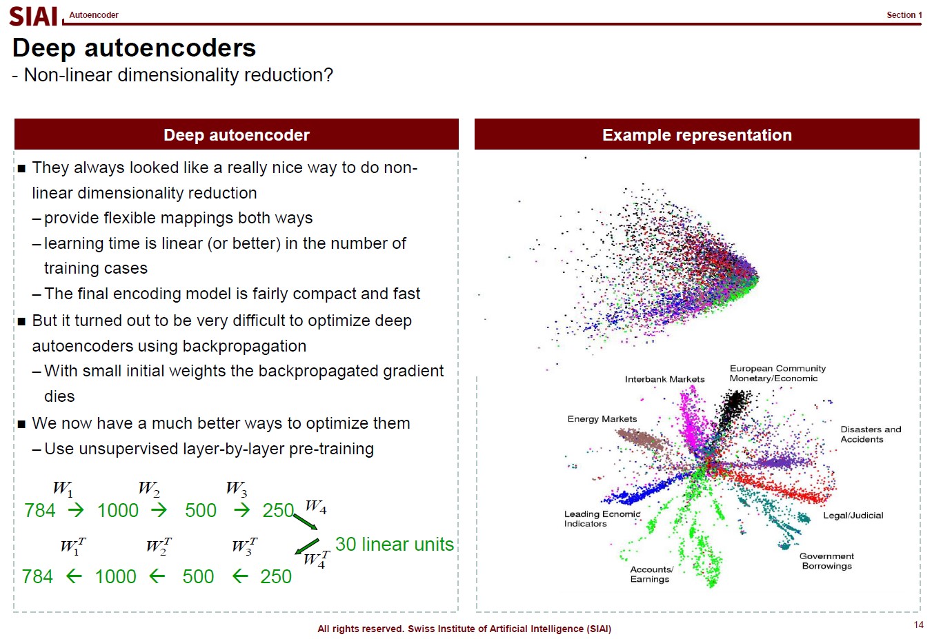
If the ‘Encoder’ is designed well, for any data that fits to your data-preprocessing for image 0 to 9, it should not be that difficult to unwind the process and recover the original data (or very close to original data). In short, it is a network version of Factor Analysis that combines ‘from’ and ‘to’.

This process is called Autoencoder, which can be used to not only for image recognifition, but it can also be used to non-linear simulation like GAN (Generative Adversarial Network).

To further optimize the painstaking encoder construction, we can borrow Bayesian estimation tactics.