Class 2. Classification

In computational science, curve fitting falls into the category of non-linear approximation. Unlilke what we have discussed in Class 1. Regression, the functional shape now has one of the two following shapes.

• Linear format for non-linear shape: $f(x) = w_0 + w_1 x + w_2 x^2 + w_3 x^3 + …$
• Non-linear format for non-linear shape: $f(x) = log(g(x))$ or $f(x) = exp(h(x))$ or any other format

Just to make the illustration simple, let’s think about simpler format, linear format. For the 3rd order function w.r.t. $x$, you need 4 parameters to be defined, which are $w_0$, $w_1$, $w_2$, and $w_3$. High school math helps us to find the values, as long as we have 4 points of the function. You need the 4th point for $w_0$, or anchor value. Then, what if the linear representation of a curve requires more than the 3rd of $x$? What if it requires 10th order of $x$? For $n$th order, we know from high school that we need at least $n+1$ points to fit the function. What if the function has infinite ups and downs? How many points do you need?

This is where we need to be smarter than high school. We need to find a pattern of the function so that we don’t have to go all the way upto $\infty$th order. This can be done if the function does have a pattern. If not, we might have to sacrifice the quality of the fit, meaning we do not aim for 100% fit.

Machine Learning is a topic that helps us to do above task, a lot more scientifically than simple trial and error.

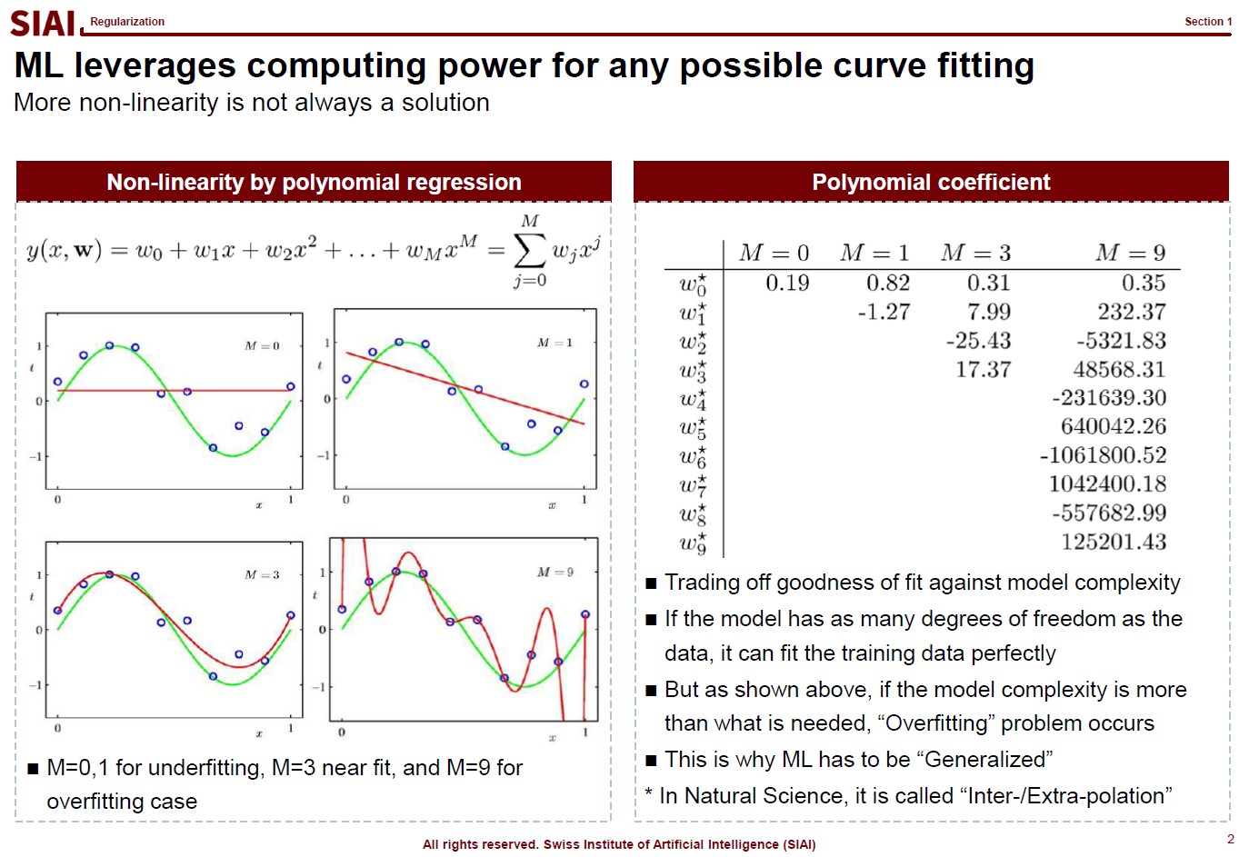
Assume that there are 10 points on the space. Except the case where 10 points are generated by a simple function (like $y=x$ or $y=x^2$), it is unlikely that we are going to end up with the perfect fit, unless we use all 10 points. The simplest linear form of the function will have 9th order of $x$ for 10 coefficients.

Let’s say you do not want to waste your time and effort for upto 9th order. It is too time consuming. You just want the 3rd order, or 4 coefficients. It will be much faster and less painful to do the calculation, but your function is unlikely going to be perfect fit. The less order you add to the function, the less accuracy you can achieve.

One may argue that it is computer that does all the calculation, then why worry about time/effort? Imagin you have to fit a function that has 1 trillion points. As the data set becomes larger, unless you have a pattern w/ lower order representation or you give up accuracy, you are going to pay large amount of computational cost. More details have already been discussed in COM501: Scientific Programming.

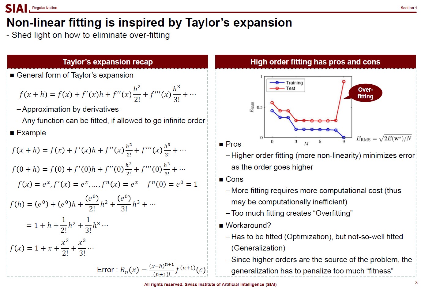
Before going deeper, let me emphasize one mathematical concept. The linear form for a curve fit is, in fact, no different from Taylor’s expansion from elementary linear algebra, at least mathematically. We often stop at 1st or 2nd order when we try to find an approximation, precisely the same reason that we do not want to waste too much computational cost for the 1 trillion points case.

And for the patterned cases like $y=sin(x)$ or $y=cos(x)$, we already know the linear form is a simple sequence. For those cases, it is not needed to have 1 trillion points for approximation. We can find the perfect fit with a concise functional form.

In other words, what machine learning does is nothing more than finding a function like $y=sin(x)$ when your data has infinite number of ups and downs in shape.

Let’s think about regularization. ML textbooks say that regularization is required to fit the function more generally while sacrificing the perfect fit for a small sample data.

Borrowing more mathematical terms, we can say that the fitting is to find the maximum optimization. ML can help us to achieve better fit or more optimization, if linear approximation is not perfect enough. This is why you often hear that ML provides better fit than traditional stat (from amateur data scientists, obviously).

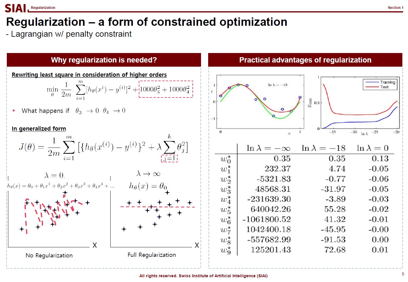
But, if the fit is limited to current sample data set only, you do not want to claim a victory. It is better to give up some optimization for better generality. The process of regularization, thus is generalization. What it does is to make the coefficients smaller in absolute value, thus make the function less sensitive to data. If you go full regularization, the function will have (near) 0 values in all coefficients, which will give you a flat line. You do not want that, after spending heavy computational cost, so the regularization process is to build a compromise between optimization and generalization.

(Note that, in the above screenshot, j starts from 1 instead of 0 ($j=1$), because $j=0$ is the level, or anchor. If you regularize the level, your function converges to $y=0$. Another component to help you to understand that regularization is just to make the coefficients smaller in absolute value.)

There are, in fact, many variations that you can create in regularization, depending on your purpose. For example, students ask me why we have to stick to quadratic format ($\theta^2$), instead of absolute value ($|\theta|$). Both cases are feasible, but for the different purposes.

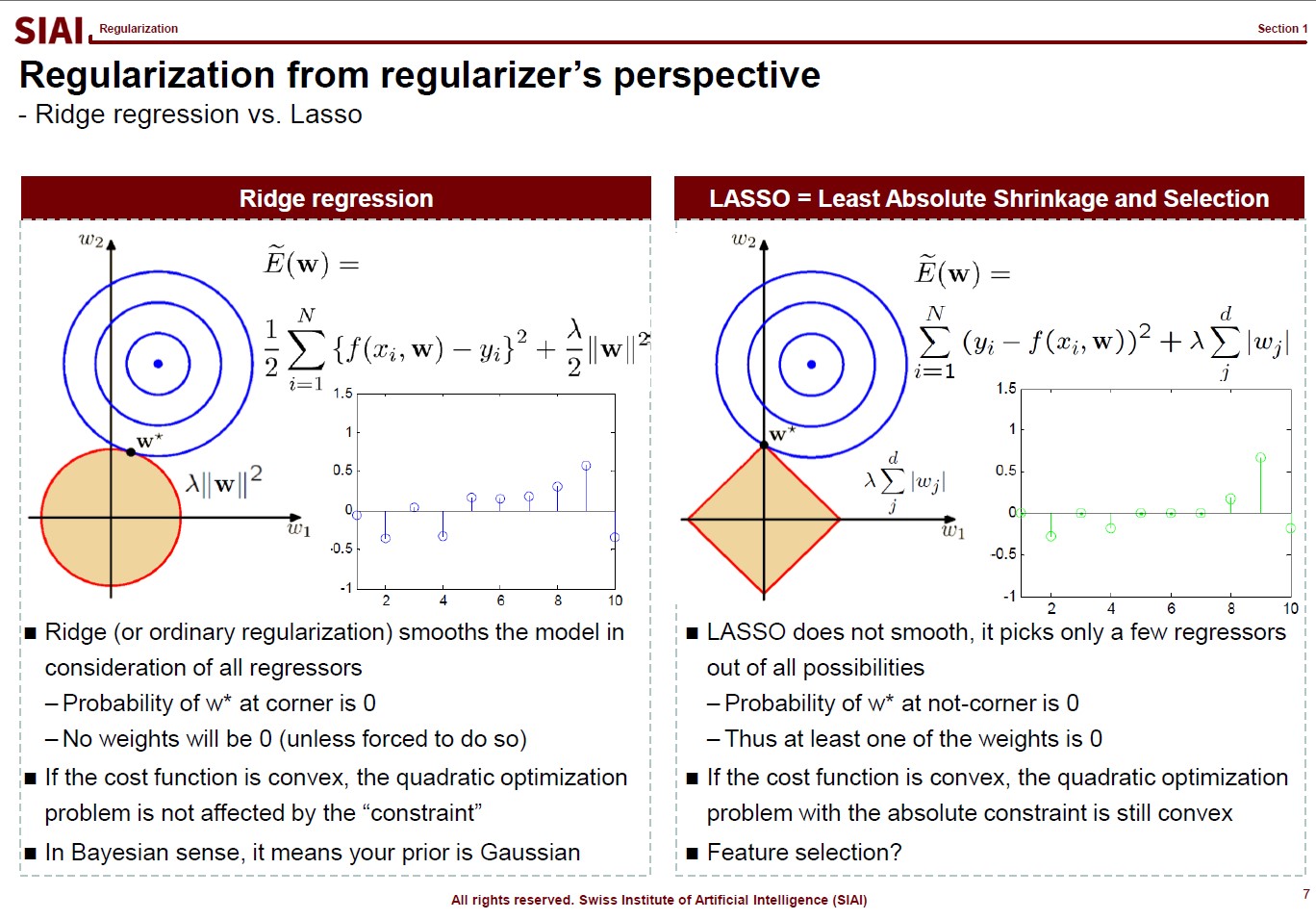
In the above lecture note, the quadratic case is coined as ‘Ridge’ and the absolute as ‘LASSO’. The quadratic case is to find a combination of $\theta_1$ and $\theta_2$, assuming it is a 2-dimensional case. Your regularization parameter ($\lambda$) will affect both $\theta_1$ and $\theta_2$. In the graphe, $w*$ has non-zero values of ($w_1$, $w_2$).

On the contrary, LASSO cases help you to isolate a single $\theta$. You choose to regularize either from $x_1$ or $x_2$, thus one of the $\theta_i$ will be 0. In the graph, as you see, $w_1 is 0.

By the math terms, we call quadratic case as L2 regularization and the absolute value case as the L1 regularization. L1 and L2 being the order of the term, in case you wonder where the name comes from.

Now assume that you change the value of $\lambda$ and $w_i$. For Ridge, there is a chance that your $w=(w_1, w_2)$ will be (0,$k$) (for $k$ being non zero), but we know that a point on a line (or a curve) carries a probability of $\frac{1}{\infty}$. In other words, for Ridge, the chance that you will end up with a single value regularization is virtually 0. It will affect jointly. But LASSO gives the opposite. From $w=(0, w_2)$, an $\epsilon$(>0) change of your parameter will take you to $w=(w_1, 0)$. Again, the probability of non-zero $w_i$s is not 0, but your regularization will not end up with that joint point.

Obviously, your real-life example may invalidate above construction in case you have missing values, your regularizers have peculiar shapes, or any other extensions. I added this slide because I’ve seen a number of amateurs simply test Ridge and LASSO and choose whatever the highest fit they end up with. Given the purpose of regularization, higher fit is no longer the selection criteria. By the math, you can see how both approaches work, so that you can explain why Ridge behaves in one way while LASSO behaves another.

Now let’s thinkg about where this L2 regularization really is rooted. If we are lucky enough, we may be able to process the same for L1.

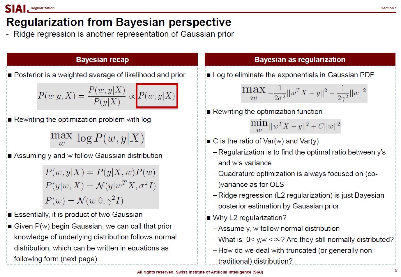
Think of an Bayesian regression. All regressions relies on the idea that given $X$, your combination of $w$ with respect to $y$ helps you to find the optimal $w$. By the conditional probability rule that we use in Bayesian decomposition, the regression can be re-illustrated as the independent joint event of $P(y|X,w)$ and $P(w)$. (Recall that $P(X, Y) = P(X) \times P(Y)$ means $X$ and $Y$ are independent events.)

If we assume both $P(y|X,w)$ and $P(w)$ normal distribution, on the right side of the above lecture note, we end up with the regularization form that we have seen a few pages earlier. In other words, the L2 regularization is the same as an assumption that our $w$ and $y|X$ follows normal distribution. If $w$ does not follow normal, the regularization part should be different. L1 means $w$ follows Laplace.

In plain English, your choice of L1/L2 regularization is based on your belief on $w$.

You hardly will rely on regularizations on a linear function, once you go to real data work, but above discussion should help you to understand that your choice of regularization should reflect your data. After all, I always tell students that the most ideal ML model is not the most fitted to current sample but most DGP* fitted one. (*DGP:Data Generating Process)

For example, if your $w$s have to be positive by DGP, but estimated $w$ are closed to 0, vanilla L2 regularization might not be the best choice. You either have to shift the value far away from 0, or rely on L1, depending on your precise assumption on your own $w$s.

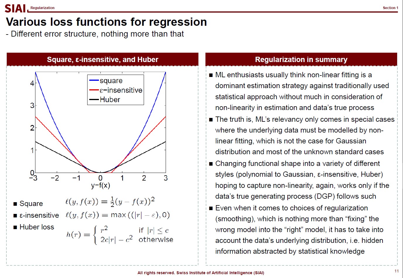
Just like your $w$ reflects your assumption that yields the quadratic form for normal distribution, your loss function also reflects your assumption on $y|X$. As before, your DGP rules what can be the best choice of loss function.

DGP matters in every estimation/approximation/fitting strategies. Many amateur data scientists claim a victory for an higher fit, but no consideration to DGP means you are just lucky to come up with a fitted model for that particular data. Unless you data is endlessly repeated, the luck may not last.

Support Vector Machine Precap – KKT (Karush-Kuhn-Tucker) method

Before we jump onto the famous SVM(Support Vector Machine) model, let’s briefly go over related math from undergrad linear algebra. If you know what Kuhn-Tucker is, skip this section and move onto the next one.

Let’s think about a simple one variable optimization case from high school math. To find the max/min points, one can rely on F.O.C. (first order condition.) For example, to find the minimum value of $y$ from $y=x^2 -2x +1$,

• Objective Function: $y= x^2 – 2x +1$
• FOC: \frac{dy}{dx} = 2x -2

The $x$ value that make the FOC equal to 0 is $x=1$. To prove if it gives us minimum value, we do the S.O.C. (second order condition).

• SOC: \frac{dy}{dx^2} = 2

The value is larger than 0, thus we can confirm the original function is convex, which has a lower bound from a range of continuous support. So far, we assumed that both $x$ and $y$ are from -$\infty$ to +$\infty$ . What if the range is limited to below 0? Your answer above can be affected depending on your solution from FOC. What if you have more than $x$ to find the optimalizing points? What if the function looks like below:

• New Objective Function: $z = x^2 -2x +1 + y^2 -2y +1$

Now you have to deal with two variables. You still rely on similar tactics from a single variable case, but the structure is more complicated. What if you have a boundary condition? What about more than one boundary conditions? What about 10+ variables in the objective function? This is where we need a generalized form, which is known as Lagrangian method where the mulivariable SOC is named as Hessian matrix. The convex/concave is positive / negative definite. To find the posi-/nega-tive definiteness, one needs to construct a Hessian matrix w/ all cross derivative terms. Other than that, the logic is unchanged, however many variables you have to add.

What becomes more concerning is when the boundary condition is present. For that, your objective function becomes:

• Bounded Objective Function: $z=x^2 -2x +1 + y^2 -2y +1 + \lambda (g(x)-k)$
  • where $g(x)-k=0$ being a boundary condition, and $\lambda$ a Lagrangian multiplier

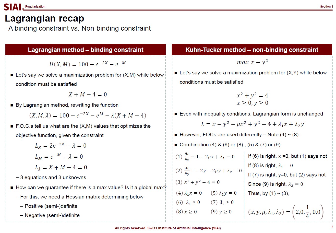
Instead of solving a two ($x$, $y$) variable problem, one just needs to solve a three ($x$, $y$, $\lambda$) variable problem. Then, what if the boundary condition is no longer given with equality($=$)? This is where you need Kuhn-Tucker technique. (An example is given in the RHS of the above lecture note screen shot).

Although the construction of the objective function with boundary condition is the same, you now need to ‘think’ to fill the gap. In the above example, from (4), one can say either $\lambda_1$ or $x$ is 0. Since you have a degree of freedom, you have to test validities of two possibilities. Say if $x=0$ and $\lambda_1>0$, then (1) does not make sense. (1) says $\lambda_1 = -1$, which contradicts with boundary condition, $\lambda_1 >0$. Therefore, we can conclude that $x>0$ and $\lambda_1=0$. With similar logic, from (5), you can rule out (7) and pick (9).

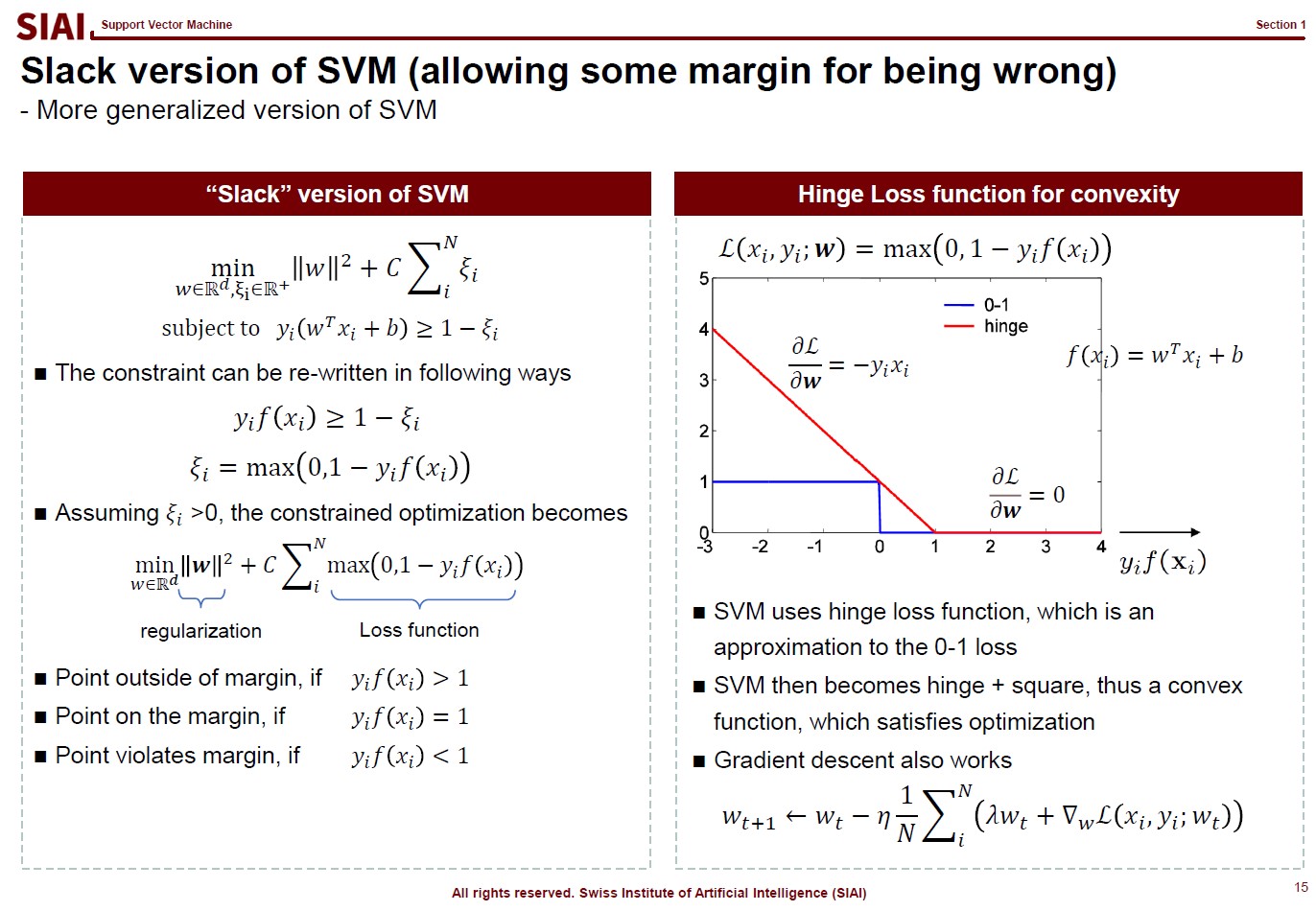
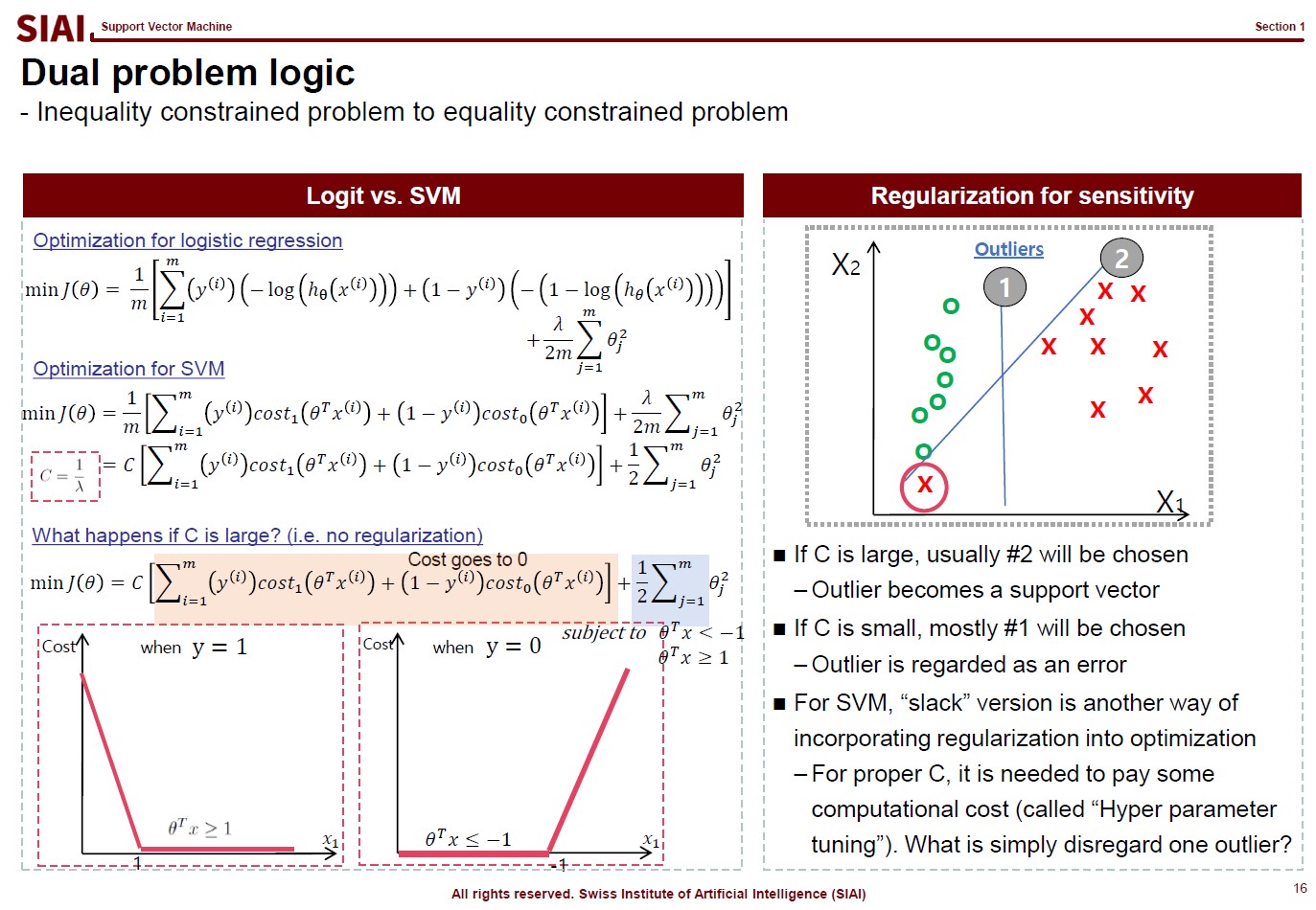
This logical process is required for inequality boundaries for Lagrangian. Why do you need this for SVM? You will later learn that SVM is a technique to find a separating hyperplane between two inequality boundary conditions.