Keith Lee is a Professor of AI and Data Science at the Gordon School of Business, part of the Swiss Institute of Artificial Intelligence (SIAI), where he leads research and teaching on AI-driven finance and data science. He is also a Senior Research Fellow with the GIAI Council, advising on the institute’s global research and financial strategy, including initiatives in Asia and the Middle East.
Input
Picture
Member for
9 months 2 weeks
Real name
Keith Lee
Bio
Keith Lee is a Professor of AI and Data Science at the Gordon School of Business, part of the Swiss Institute of Artificial Intelligence (SIAI), where he leads research and teaching on AI-driven finance and data science. He is also a Senior Research Fellow with the GIAI Council, advising on the institute’s global research and financial strategy, including initiatives in Asia and the Middle East.
Keith Lee is a Professor of AI and Data Science at the Gordon School of Business, part of the Swiss Institute of Artificial Intelligence (SIAI), where he leads research and teaching on AI-driven finance and data science. He is also a Senior Research Fellow with the GIAI Council, advising on the institute’s global research and financial strategy, including initiatives in Asia and the Middle East.
Input
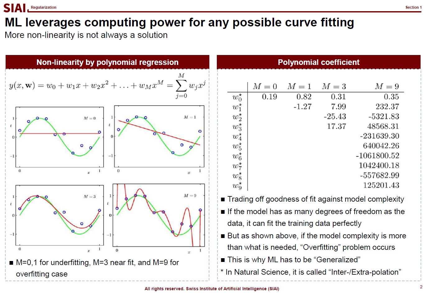
In computational science, curve fitting falls into the category of non-linear approximation. Unlilke what we have discussed in Class 1. Regression, the functional shape now has one of the two following shapes.
Linear format for non-linear shape: $f(x) = w_0 + w_1 x + w_2 x^2 + w_3 x^3 + ...$
Non-linear format for non-linear shape: $f(x) = log(g(x))$ or $f(x) = exp(h(x))$ or any other format
Just to make the illustration simple, let's think about simpler format, linear format. For the 3rd order function w.r.t. $x$, you need 4 parameters to be defined, which are $w_0$, $w_1$, $w_2$, and $w_3$. High school math helps us to find the values, as long as we have 4 points of the function. You need the 4th point for $w_0$, or anchor value. Then, what if the linear representation of a curve requires more than the 3rd of $x$? What if it requires 10th order of $x$? For $n$th order, we know from high school that we need at least $n+1$ points to fit the function. What if the function has infinite ups and downs? How many points do you need?
This is where we need to be smarter than high school. We need to find a pattern of the function so that we don't have to go all the way upto $\infty$th order. This can be done if the function does have a pattern. If not, we might have to sacrifice the quality of the fit, meaning we do not aim for 100% fit.
Machine Learning is a topic that helps us to do above task, a lot more scientifically than simple trial and error.
Assume that there are 10 points on the space. Except the case where 10 points are generated by a simple function (like $y=x$ or $y=x^2$), it is unlikely that we are going to end up with the perfect fit, unless we use all 10 points. The simplest linear form of the function will have 9th order of $x$ for 10 coefficients.
Let's say you do not want to waste your time and effort for upto 9th order. It is too time consuming. You just want the 3rd order, or 4 coefficients. It will be much faster and less painful to do the calculation, but your function is unlikely going to be perfect fit. The less order you add to the function, the less accuracy you can achieve.
One may argue that it is computer that does all the calculation, then why worry about time/effort? Imagin you have to fit a function that has 1 trillion points. As the data set becomes larger, unless you have a pattern w/ lower order representation or you give up accuracy, you are going to pay large amount of computational cost. More details have already been discussed in COM501: Scientific Programming.
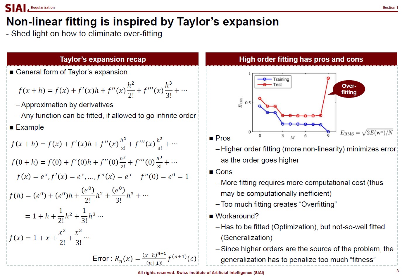
Before going deeper, let me emphasize one mathematical concept. The linear form for a curve fit is, in fact, no different from Taylor's expansion from elementary linear algebra, at least mathematically. We often stop at 1st or 2nd order when we try to find an approximation, precisely the same reason that we do not want to waste too much computational cost for the 1 trillion points case.
And for the patterned cases like $y=sin(x)$ or $y=cos(x)$, we already know the linear form is a simple sequence. For those cases, it is not needed to have 1 trillion points for approximation. We can find the perfect fit with a concise functional form.
In other words, what machine learning does is nothing more than finding a function like $y=sin(x)$ when your data has infinite number of ups and downs in shape.
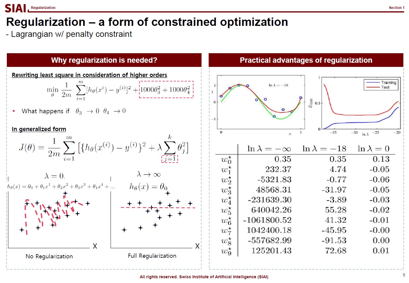
Let's think about regularization. ML textbooks say that regularization is required to fit the function more generally while sacrificing the perfect fit for a small sample data.
Borrowing more mathematical terms, we can say that the fitting is to find the maximum optimization. ML can help us to achieve better fit or more optimization, if linear approximation is not perfect enough. This is why you often hear that ML provides better fit than traditional stat (from amateur data scientists, obviously).
But, if the fit is limited to current sample data set only, you do not want to claim a victory. It is better to give up some optimization for better generality. The process of regularization, thus is generalization. What it does is to make the coefficients smaller in absolute value, thus make the function less sensitive to data. If you go full regularization, the function will have (near) 0 values in all coefficients, which will give you a flat line. You do not want that, after spending heavy computational cost, so the regularization process is to build a compromise between optimization and generalization.
(Note that, in the above screenshot, j starts from 1 instead of 0 ($j=1$), because $j=0$ is the level, or anchor. If you regularize the level, your function converges to $y=0$. Another component to help you to understand that regularization is just to make the coefficients smaller in absolute value.)
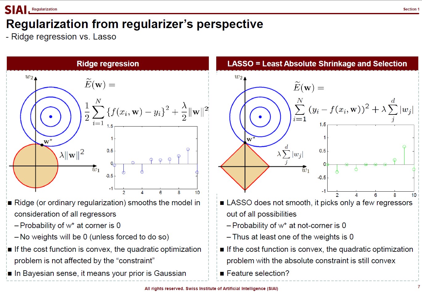
There are, in fact, many variations that you can create in regularization, depending on your purpose. For example, students ask me why we have to stick to quadratic format ($\theta^2$), instead of absolute value ($|\theta|$). Both cases are feasible, but for the different purposes.
In the above lecture note, the quadratic case is coined as 'Ridge' and the absolute as 'LASSO'. The quadratic case is to find a combination of $\theta_1$ and $\theta_2$, assuming it is a 2-dimensional case. Your regularization parameter ($\lambda$) will affect both $\theta_1$ and $\theta_2$. In the graphe, $w*$ has non-zero values of ($w_1$, $w_2$).
On the contrary, LASSO cases help you to isolate a single $\theta$. You choose to regularize either from $x_1$ or $x_2$, thus one of the $\theta_i$ will be 0. In the graph, as you see, $w_1 is 0.
By the math terms, we call quadratic case as L2 regularization and the absolute value case as the L1 regularization. L1 and L2 being the order of the term, in case you wonder where the name comes from.
Now assume that you change the value of $\lambda$ and $w_i$. For Ridge, there is a chance that your $w=(w_1, w_2)$ will be (0,$k$) (for $k$ being non zero), but we know that a point on a line (or a curve) carries a probability of $\frac{1}{\infty}$. In other words, for Ridge, the chance that you will end up with a single value regularization is virtually 0. It will affect jointly. But LASSO gives the opposite. From $w=(0, w_2)$, an $\epsilon$(>0) change of your parameter will take you to $w=(w_1, 0)$. Again, the probability of non-zero $w_i$s is not 0, but your regularization will not end up with that joint point.
Obviously, your real-life example may invalidate above construction in case you have missing values, your regularizers have peculiar shapes, or any other extensions. I added this slide because I've seen a number of amateurs simply test Ridge and LASSO and choose whatever the highest fit they end up with. Given the purpose of regularization, higher fit is no longer the selection criteria. By the math, you can see how both approaches work, so that you can explain why Ridge behaves in one way while LASSO behaves another.
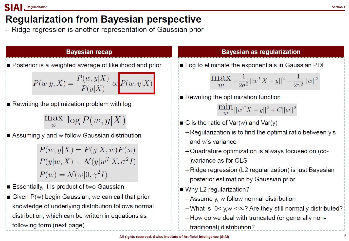
Now let's thinkg about where this L2 regularization really is rooted. If we are lucky enough, we may be able to process the same for L1.
Think of an Bayesian regression. All regressions relies on the idea that given $X$, your combination of $w$ with respect to $y$ helps you to find the optimal $w$. By the conditional probability rule that we use in Bayesian decomposition, the regression can be re-illustrated as the independent joint event of $P(y|X,w)$ and $P(w)$. (Recall that $P(X, Y) = P(X) \times P(Y)$ means $X$ and $Y$ are independent events.)
If we assume both $P(y|X,w)$ and $P(w)$ normal distribution, on the right side of the above lecture note, we end up with the regularization form that we have seen a few pages earlier. In other words, the L2 regularization is the same as an assumption that our $w$ and $y|X$ follows normal distribution. If $w$ does not follow normal, the regularization part should be different. L1 means $w$ follows Laplace.
In plain English, your choice of L1/L2 regularization is based on your belief on $w$.
You hardly will rely on regularizations on a linear function, once you go to real data work, but above discussion should help you to understand that your choice of regularization should reflect your data. After all, I always tell students that the most ideal ML model is not the most fitted to current sample but most DGP* fitted one. (*DGP:Data Generating Process)
For example, if your $w$s have to be positive by DGP, but estimated $w$ are closed to 0, vanilla L2 regularization might not be the best choice. You either have to shift the value far away from 0, or rely on L1, depending on your precise assumption on your own $w$s.
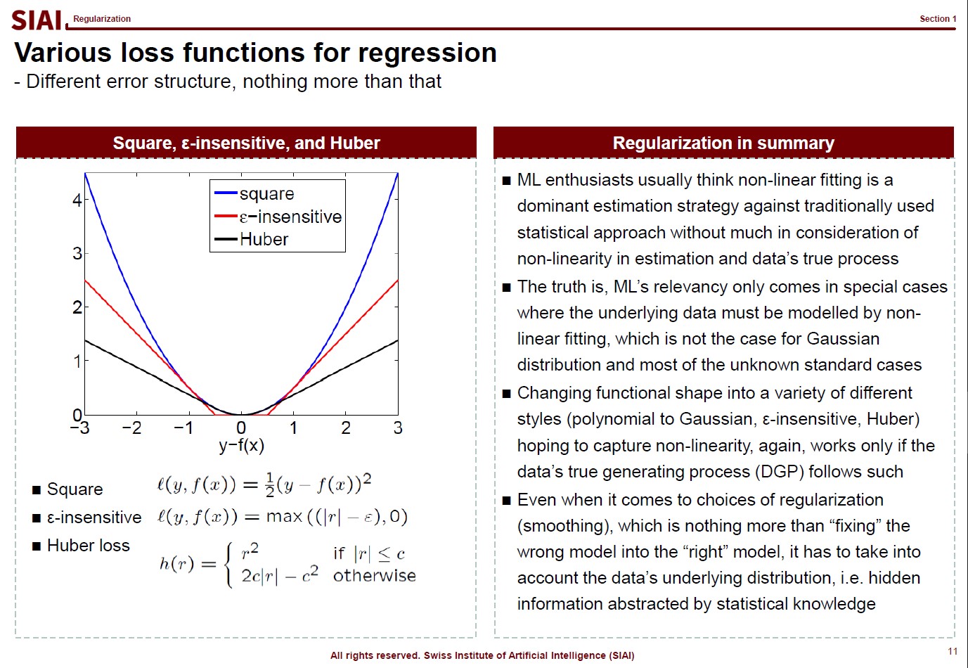
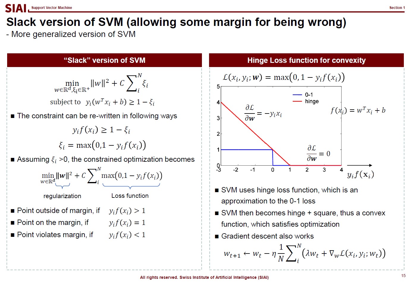
Just like your $w$ reflects your assumption that yields the quadratic form for normal distribution, your loss function also reflects your assumption on $y|X$. As before, your DGP rules what can be the best choice of loss function.
DGP matters in every estimation/approximation/fitting strategies. Many amateur data scientists claim a victory for an higher fit, but no consideration to DGP means you are just lucky to come up with a fitted model for that particular data. Unless you data is endlessly repeated, the luck may not last.
Support Vector Machine Precap - KKT (Karush-Kuhn-Tucker) method
Before we jump onto the famous SVM(Support Vector Machine) model, let's briefly go over related math from undergrad linear algebra. If you know what Kuhn-Tucker is, skip this section and move onto the next one.
Let's think about a simple one variable optimization case from high school math. To find the max/min points, one can rely on F.O.C. (first order condition.) For example, to find the minimum value of $y$ from $y=x^2 -2x +1$,
Objective Function: $y= x^2 - 2x +1$
FOC: $\frac{dy}{dx} = 2x -2$
The $x$ value that make the FOC equal to 0 is $x=1$. To prove if it gives us minimum value, we do the S.O.C. (second order condition).
SOC: $\frac{dy}{dx^2} = 2$
The value is larger than 0, thus we can confirm the original function is convex, which has a lower bound from a range of continuous support. So far, we assumed that both $x$ and $y$ are from -$\infty$ to +$\infty$ . What if the range is limited to below 0? Your answer above can be affected depending on your solution from FOC. What if you have more than $x$ to find the optimalizing points? What if the function looks like below:
Now you have to deal with two variables. You still rely on similar tactics from a single variable case, but the structure is more complicated. What if you have a boundary condition? What about more than one boundary conditions? What about 10+ variables in the objective function? This is where we need a generalized form, which is known as Lagrangian method where the mulivariable SOC is named as Hessian matrix. The convex/concave is positive / negative definite. To find the posi-/nega-tive definiteness, one needs to construct a Hessian matrix w/ all cross derivative terms. Other than that, the logic is unchanged, however many variables you have to add.
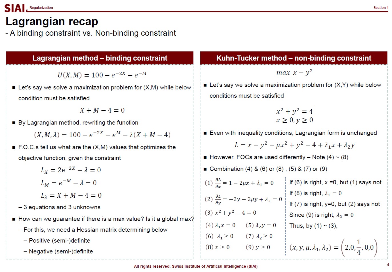
What becomes more concerning is when the boundary condition is present. For that, your objective function becomes:
where $g(x)-k=0$ being a boundary condition, and $\lambda$ a Lagrangian multiplier
Instead of solving a two ($x$, $y$) variable problem, one just needs to solve a three ($x$, $y$, $\lambda$) variable problem. Then, what if the boundary condition is no longer given with equality($=$)? This is where you need Kuhn-Tucker technique. (An example is given in the RHS of the above lecture note screen shot).
Although the construction of the objective function with boundary condition is the same, you now need to 'think' to fill the gap. In the above example, from (4), one can say either $\lambda_1$ or $x$ is 0. Since you have a degree of freedom, you have to test validities of two possibilities. Say if $x=0$ and $\lambda_1>0$, then (1) does not make sense. (1) says $\lambda_1 = -1$, which contradicts with boundary condition, $\lambda_1 >0$. Therefore, we can conclude that $x>0$ and $\lambda_1=0$. With similar logic, from (5), you can rule out (7) and pick (9).
This logical process is required for inequality boundaries for Lagrangian. Why do you need this for SVM? You will later learn that SVM is a technique to find a separating hyperplane between two inequality boundary conditions.
Picture
Member for
9 months 2 weeks
Real name
Keith Lee
Bio
Keith Lee is a Professor of AI and Data Science at the Gordon School of Business, part of the Swiss Institute of Artificial Intelligence (SIAI), where he leads research and teaching on AI-driven finance and data science. He is also a Senior Research Fellow with the GIAI Council, advising on the institute’s global research and financial strategy, including initiatives in Asia and the Middle East.
Keith Lee is a Professor of AI and Data Science at the Gordon School of Business, part of the Swiss Institute of Artificial Intelligence (SIAI), where he leads research and teaching on AI-driven finance and data science. He is also a Senior Research Fellow with the GIAI Council, advising on the institute’s global research and financial strategy, including initiatives in Asia and the Middle East.
Input
Many people think machine learning is some sort of magic wand. If a scholar claims that a task is mathematically impossible, people start asking if machine learning can make an alternative. The truth is, as discussed from all pre-requisite courses, machine learning is nothing more than a computer version of statistics, which is a discipline that heavily relies on mathematics.
Once you step aside from basic statistical concepts, such as mean, variance, co-variance, and normal distribution, all statistical properties are built upon mathematical language. In fact, unless it is purely based on experiments, mathematics is a language of science. Statistics as a science is no exception. And, machine learning is a computational approach of statistics, which we call computational statistics.
Throughout this course, it is introduced that all machine learning topics are deeply based on statistical properties. Although the SIAI's teaching relies less on math more on practical applications, it is still required to learn key mathematical backgrounds, if to use machine learning properly. If you skip this part, then you will be one of the amateurs arguing machine learning (or any computational statistical sub-disciplines) as a magic.
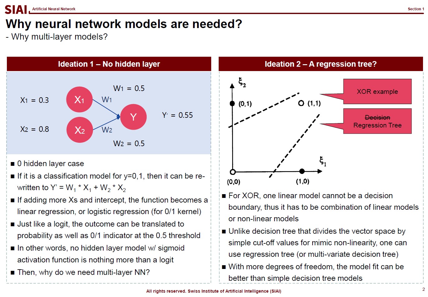
When do you need machine learning?
To answer why machine learning become suddenly popular, you first have to understand what it really does. Machine learning helps us to find a non-parametric function that fits to data. Non-parametric means that you do not have a specific functional shape, like $y=a \cdot x^2 + b \cdot x + c$. Once you step away from linear representation of the function, there can be infinite number of possibilities to represent a function. $y=f(x)$ can be a combination of exponential, log, or any other form you want. As long as it fits to data, why care so much?
Back then, fitting to data was only the first agenda. Because the data in your hand is only a sample of the giant population. For example, if a guy claim that he can perfectly match stock price movements for the last 3 years for a specific stock. Then, amateurs are going to ask him if
The horizon can be expanded not only to the distant past, but also for the future
Other stock prices can be replicated
If the stock price returns are randome, a fit for sample data cannot be replicated to other sets of data, unless miracle occurs. In mathematical terms, we call it a probability $\frac{1}{\infty}$ event. If you have done some stochastic calculus, it can be said that the probability converges to 0 almost surely (a.s.).
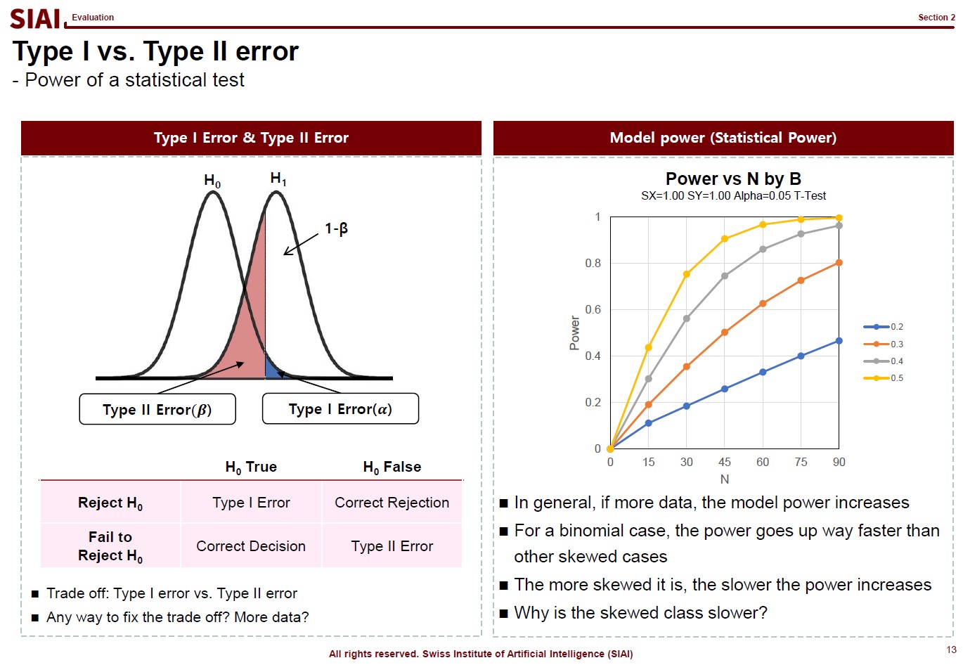
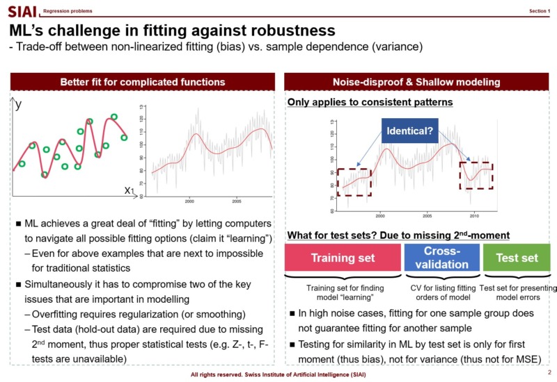
Here, the second agenda arises, which is minimizing model variance for generality of the model. In statistics, it is often done by Z-test, t-test, $\chi^2$-test, and F-test. Although the statistical tests based on (co-)variance (or 2nd-moments, in more scientific terms) is not universal solution to claim generality of the model, if conditions fit, we can argue that it is fairly good enough. (Conditions that can be satisfied if you data follows normal distribution, for example).
Unfortunately, machine learning hardly addresses the second one. Why? Because machine learning relies on further assumptions. The 2nd-moment should be irrelevant for it to work. What are the data sets that overrules the 2nd-moment tests? Data that does not follow random distribution, thus does not have variance. Data that follows rules.
In short, machine learning is not for random data. The quest to find an ultra complicated function should be rewarding, and the probability is guaranteed if such funcational events are highly frequent. Examples of such events are like language. You do not speak random gibberish for daily conversation. (Assuming that you do not read this text in a psychiatric hospital.) As long as your language has a grammar and a dictionary for vacabulary, that means there is a rule and it is repeated, thus highly frequent.
Then, how come machine learning become so popular?
Out of many other reasons that machine learning suddenly becomes popular, one thing that can be told is that we now have a plethora of highly frequent data with certain rules. You do not need bigtech companies to build a peta-byte database of text, image, and any other contents with rules. Finding a linear functional form, like $y=a \cdot x^2 + b \cdot x + c$, for such data is mostly next to impossible. Then, what is an ideal alternative? Is there any alternative? Remember that machine learning helps us to fit such a complicated function.
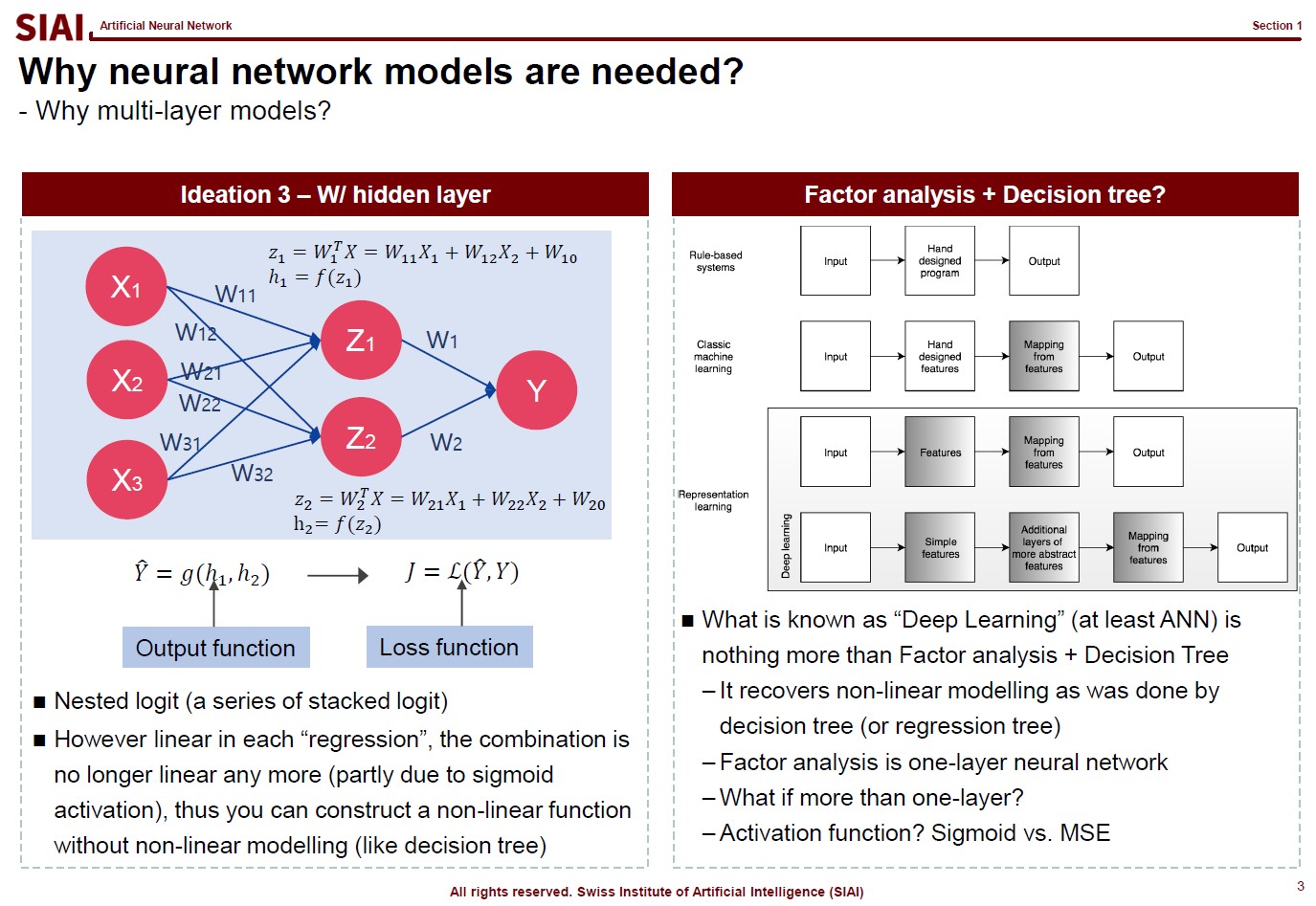
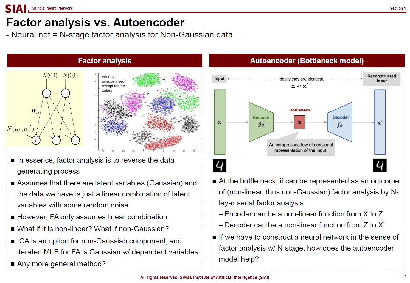
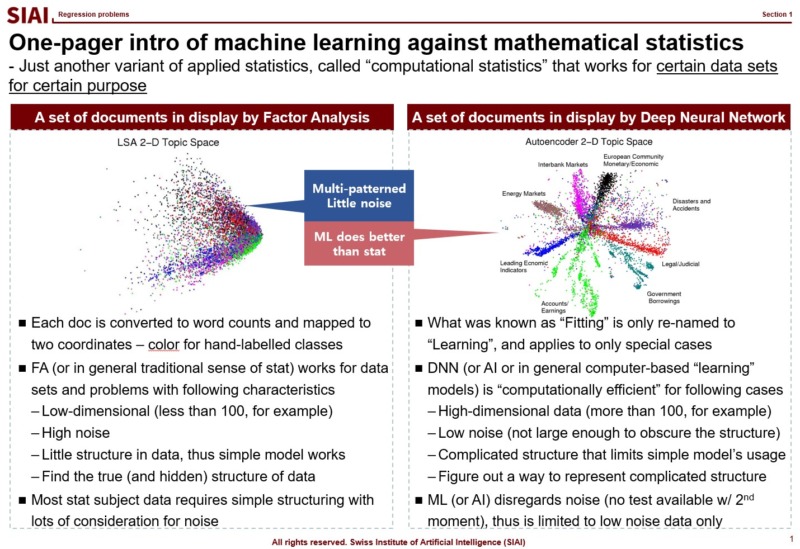
The first page of this lecture note then starts with an example of traditional statistics that fails to find such a function. In the above screenshot, on the left, factor analysis cannot help us to differentiate data sets of 0~9. There are 10 types of data, but factor analysis was not able to find key characteristics of each type. It is because the combination of characters are complicated, and a simple function cannot find the decent fit. For example, number 3 and 9 have the similar shape on the upper right part and bottom center part. Number 5 and 9 have the similar bottom right part. Number 0 and 9 also share the upper right part and the bottom right part. You need more than a simple function to match all combinations. This is where multi-layer factor analysis (called Deep Neural Network) can help us.
Throughout the course, just like above, each machine learning topic will be introduced in a way to overcome given trouble that traditional statistics may not solve easily. Note that it does not mean that machine learning is superior to traditional statistics. It just helps us to find a highly non-linear function, if your computer can do the calculation. Possibilities are still limited and often explained in mathematical format. In fact, all machine learning jargons have more scientific alternative, like multi-layer factor analysis to Deep Neural Network, which also means there is a scientific back-up needed to fully understand what it really does. Again, computational methods are not magic. If you want to wield the magic wand properly, you have to learn the language of the 'magic', which is 'mathematics'.
Most simpliest possible machine learning is to find a non-linear fit of a data set. As you have more and more data points, the function to match all points is necessarily going to have more ups and downs, unless you have a data set fits to a linear function. Thus, if you have more data, it is likely that you are going to suffer from less fit with abundant error or more fit with complication in function.
As discussed above, machine learning approaches are to find a fit, or 1st-moment (mean, average, min, max...), which assumes that data set is repeated in out of sample. As long as it fits to data in hand, machine learning researchers assume that it fits to all other data in the same category. (This is why a lot of engineers, after the 1st lecture of machine learning, claim that they can find a fit to stock price movements and make money in the market. They don't understand that financial markets are full of randomness.)
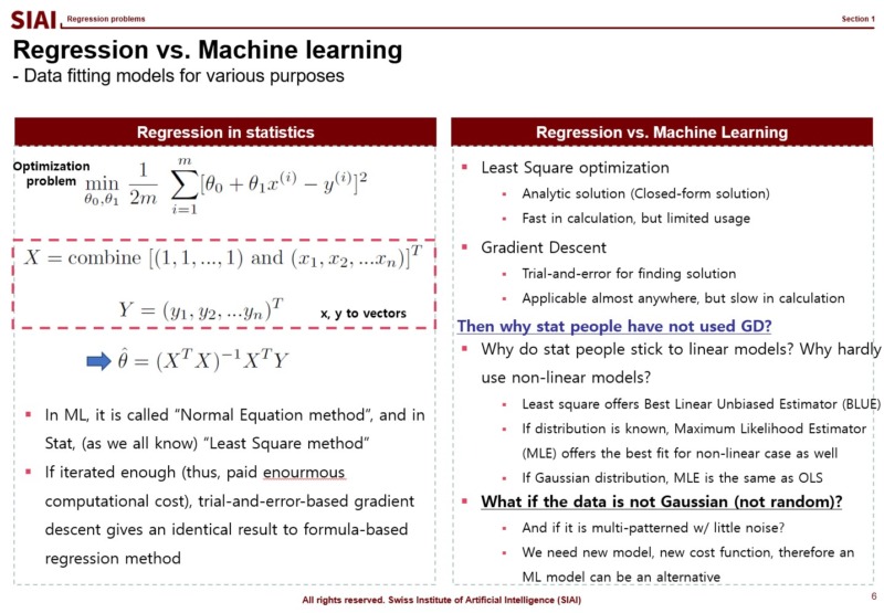
In statistics, the simplest form of regression is called ordinary least square (OLS). In machine learning, the OLS solution is called 'Normal equation' method. Why are they end up with the same form of the solution?
This happens only when the OLS is the most optimal fit to given data set, which is coined as 'Best Linear Unbiased Estimator (BLUE)' in statistics, where one condition for OLS to be BLUE is the target variable follows normal distribution. To be precise, statistians say that $y$ is normally distributed conditional on $X$, or $y|X \backsim N(\beta \cdot X, \sigma^2)$. Given your explanatory variables, if your target variable follows normal distribution, your machine learning model will give you exactly the same solution as OLS. In other words, if you have normally distributed random data, then you don't have to go for machine learning models to find the optimal fit. You need machine learning models when your target variable is not normally distributed, and it is not random.
Just to note that if your data follows a known distribution, like Poisson, Laplace, Binomial..., there is a closed-form BLUE solution, so don't waste your computational cost for machine learning. It's like high school factorization. If you know the form, you have the solution right away. If not, you have to rely on a calculator. For questions like $x^2 - 2x +1 =0$ is simple, but complicated questions may require enourmous amount of computational cost. You being smart is the key cost saving for your company.
In real world, hardly any data (except natural language and image) have non-distributional approximation. Most data have proxy distribution, which gives near optimal solution with known statistics. This is why elementary statistics only teach binomial (0/1) and Gaussian ($N(\mu, \sigma^2)$)distribution cases. Remember, machine learning is a class of non-parametric computational approach. It is to find a fit that matches to unknown function. And, it does not give us variance for testing. The entire class of machine learning models assume that there are strong patterns in the data set, otherwise a model without out of sample property is not a model. It is just a waste of computer resource.
Think of an engineer claiming that he can forecast stock price movements based on previous 3 years data. He may have a perfect fit, after running a computational model for years (or a lot of electric power and super expensive graphics card.) We know that stock prices are deeply exposed to random components, which means that his model will not fit for the next 3 years. What would you call the machine learning model? He may claim that he needs more data or more computational power. Financial economists would call them amateurs, if not idiots.
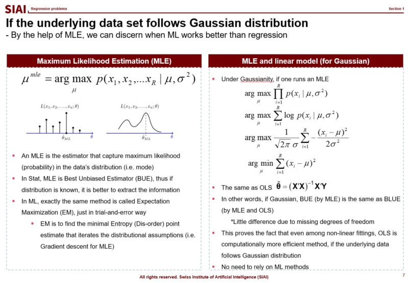
Then, one may wonder, what about data sets that fit better with non-linear model? In statistics, maximum likelihood estimators (MLE) are known as the best unbiased estimator (BUE), as long as the distributional shape is known. And, if the distribution is normal, as discussed in earlier slides, it matches exactly the same as OLS. (Note that variance is slightly different due to loss of degrees of freedom, but $N-1$ and $N$ are practically the same, if $N \rightarrow \infty$.)
In general, if the model is limited to linear class models, simple OLS (or GLS, at best) is the optimal approach. If the distributional shape is known, MLE i the best option. If your data does not have known distribution, but needs to find a definitive non-linear pattern, that's when you need to run machine learning algorithms.
Many amateurs blatantly run machine learning models and claim that they found the most fitted solution, like accuracy rate is 99.99%. As discussed, with machine learning, you cannot do any out of sample test. You might be 99.99% accurate for today's data, but you cannot guarantee that tomorrow. Borrowing the concept of computational efficiency from COM501:Scientific Programming, machine learning models are exposed to larger MSE and more computational cost. Therefore, for data sets OLS and MLE are the best fit, all machine learning models are inferior.
Above logic is the centerpiece of COM502: Machine Learning, and in fact is the single most important point of the entire program at SIAI. Going forward, for every data problem that you have, the first question you have to answer is if you need to rely on machine learning models. If you stick to it despite random data set closed to Gaussian distribution, you are a disqualified data scientist.
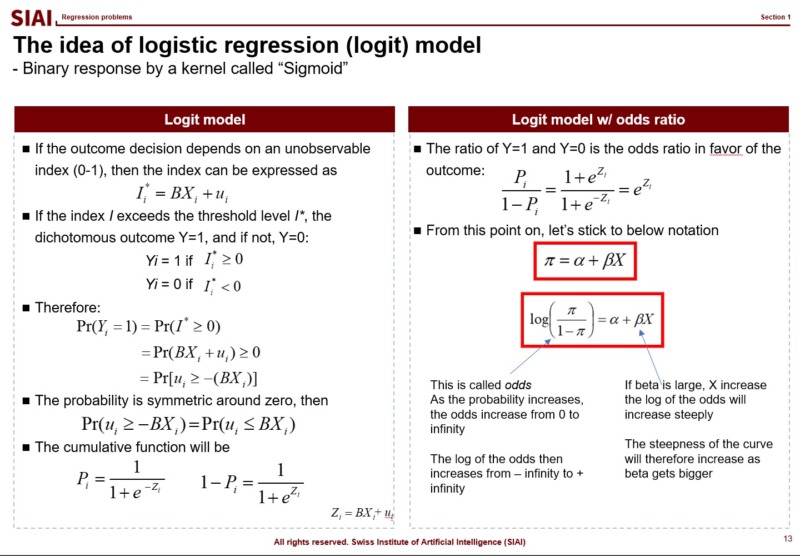
Kernel function for 0/1 or 0~100 scale
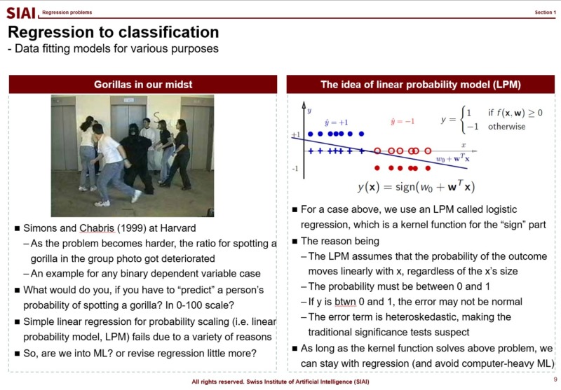
What if the outcome that you have to find the fit is no longer a continuous value from 0 to 100, or -$\infty$ to $\infty$? In mathematics, we call this as 'support', meaning that your value's range. in other words, by the mathematical jargon, if your target variable's support is 0/1 or Yes/No, your strategy might be affected, because you no longer have to match a random variable following normal distribution. We call 0/1 value cases as 'binomial distribution', and it requires different approximation strategy.
One that has been widely used is to apply a kernel function, which transforms your value to another support. From your high school math, you should have come across $y=f(x)$, (if not, your trial to learn ML is likely going to be limited to code copying only), a simplest form that tells us that $x$ is transformed to $y$ by function $f$. The function can be anything, as long as it converts $x$ to $y$, without any slag. (Mathematically, we call that $f$ is defined on $x$.)
If the transformation function $f$ maps value $x$ to 0~1, or Yes/No, we can fit Yes/No cases, just like we did with normal distribution.
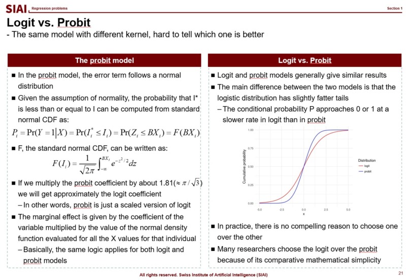
There are two widely adapted transformation $f$, Logit and Probit. As you can see from above lecture note, Logit coverts the $x$ value by odds ratio. Unfortunately, there is no closed form solution to calculate the ratio with hands, so we follow Newton methods, which we learned from COM501: Scientific Programming. The approach relies on the idea that likelihood of the value to be 0 vs. ths same probability to be 1. The ratio can be varying from -$\infty$ to +$\infty$, but the re-scaling put it into 0~1 frame.
Similarly, Probit transforms the outcome by assuming that it follows normal distribution. There is little to no difference between these two methods, when it comes to the accuracy, if you have large number of independent sample data. In small samples, usually Logit provides smoother value changes than Probit. You had more details of Logit in COM501: Scientific Programming. Check the notes.
Picture
Member for
9 months 2 weeks
Real name
Keith Lee
Bio
Keith Lee is a Professor of AI and Data Science at the Gordon School of Business, part of the Swiss Institute of Artificial Intelligence (SIAI), where he leads research and teaching on AI-driven finance and data science. He is also a Senior Research Fellow with the GIAI Council, advising on the institute’s global research and financial strategy, including initiatives in Asia and the Middle East.
Post hoc, ergo propter hoc - impossible challenges in finding causality in data science
Picture
Member for
8 months 2 weeks
Real name
David O'Neill
Bio
David O’Neill is a Professor of Finance and Data Analytics at the Gordon School of Business, SIAI. A Swiss-based researcher, his work explores the intersection of quantitative finance, AI, and educational innovation, particularly in designing executive-level curricula for AI-driven investment strategy. In addition to teaching, he manages the operational and financial oversight of SIAI’s education programs in Europe, contributing to the institute’s broader initiatives in hedge fund research and emerging market financial systems.
Published
Modified
Data Science can find correlation but not causality
In stat, no causal but high correlation is called 'Spurious regression'
Hallucinations in LLMs are repsentative examples of spurious correlation
Imagine two twin kids living in the neighborhood. One prefers to play outside day and night, while the other mostly sticks to his video games. After a year later, doctors find that the gamer boy is much healthier, thus conclude that playing outside is bad for growing children's health.
What do you think of the conclusion? Do you agree with the conclusion?
Even without much scientific training, we can almost immediately dismiss the conclusion that is based on lop-sided logic and possibly driven by insufficient information of the neighborhood. For example, if the neighborhood is as radioactively contained as Chernobyl or Fukushima, playing outside can undoubtedly be as close as committing a suicide. What about more nutrition provided to the gamer boy due to easier access to home food? The gamer body just had to drop the game console for 5 seconds to eat something, but his twin had to walk or run for 5 minites to come back home for food.
In fact, there are infinitely many potential variables that may have affected two twin kids' condition. Just by the collected data set above, the best we can tell is that for an unknown reason, the gamer boy is medically healthier than the other twin.
In more scientific terms, it can be said that statistics has been known for correlations but not for causality. Even in a controlled environment, it is hard to argue that the control variable was the cause of the effect. Researchers only 'guess' that the correlation means causality.
Post Hoc, Ergo Propter Hoc
There is a famous Latin phrase meaning "after this, therefore on account of it". In plain English, it means that one event is the cause of the other event occuring right next. You do not need rocket science to counterargue that two random events are interconnected just because one occured right after another. This is a widely common logical mistake that assigns causality just by an order of events.
In statistics, it is often called that 'Correlation does not necessarily guarantee causality'. In the same context, such a regression is called 'Spurious regression', which has been widely reported in engineers' adaptation of data science.
One noticeable example is 'Hallucination' cases in ChatGPT. The LLM only finds higher correlation between two words, two sentences, and two body of texts (or images in these days), but it fails to discern the causal relation embedded in the two data sets.
Statistians have long been working on to differentiate the causal cases from high correlation, but the best so far we have is 'Granger causallity', which only helps us to find no causality case between 3 variables. Granger causality offers a philophical frame that can help us to test if the 3rd variable can be a potential cause of the hidden causality. The academic countribution by Professor Granger's research to be Nobel Prize awarded is because it proved that it is mechanically (or philosophically) impossible to verify a causal relationship just by correlation.
Why AI ultimately needs human approval?
The Post Hoc Fallacy, by nature of current AI models, is an unavoidable huddle that all data scientists have to suffer from. Unlike simple regression based researches, the LLMs rely on too large chunk of data that it is practically impossible to tackle every connection of two text bodies.
This is where human approval is required, unless the data scientists decide to finetune the LLM in a way to offer only the highest probable (thus causal) matches. The more likely the matches are, the less likely there will be spurious connection between two sets of information, assuming that the underlying data is sourced from accurate providers.
Teaching AI/Data science, I surprisingly often come across a number of 'fake experts' whose only understanding of AI is a bunch of terminology from newspapers, or a few lines of media articles at best, without any in-depth training in basic academic tools, math and stat. When I raise Grange causality as my counterargument for impossibility to distinguish from correlation to causality by statistical methods alone (by far philosophically impossible), many of them ask, "Then, wouldn't it be possible with AI?"
If the 'fake experts' had some elementary level math and stat training from undergrad, I believe they should be able to understand that computational science (academic name of AI) is just a computer version of statistics. AI is actually nothing more than the task of performing statistics more quickly and effectively using computer calculations. In other words, AI is a sub-field of statistics. Their questions can be framed like
If it is impossible with statistics, wouldn’t it be possible with statistics calculated by computers?
If it is impossible with elementary arithmetic, wouldn't it be possible with addition and subtraction?
The inability of statistics to make causal inferences is the same as saying that it is impossible to mechanically eliminate hallucinations in ChatGPT. Those with academic training in the fields social sciences, the disciplines of which collect potentially correlated variables and use human experience as the final step to conclude causal relationships, see that ChatGPT is built to mimic cognitive behavior at the shamefully shallow level. The fact that ChatGPT depends on 'Human Feedback' in its custom version of 'Reinforcement Learning' is the very example of the basic cognitive behavior. The reason that we still cannot call it 'AI' is because there is no automatic rule for the cheap copy to remove the Post Hoc Fallacy, just like Clive Granger proved in his work for Nobel Prize.
Causal inference is not monotonically increasing challenge, but multi-dimensional problem
In natural science and engineering, where all conditions are limited and controlled in the lab (or by a machine), I often see cases where they see human correction as unscientific. Is human intervention really unscientific? Well, Heidelberg's indeterminacy principle states that when a human applies a stimulus to observe a microscopic phenomenon, the position and state just before applying the stimulus can be known, but the position after the stimulus can only be guessed. If no stimulation is applied at all, the current location and condition cannot be fully identified. In the end, human intervention is needed to earn at least partial information. Withou it, one can never have any scientifically proven information.
Computational science is not much different. In order to rule out hallucinations, researchers either have to change data sets or re-parameter the model. The new model may be closer to perfection for that particular purpose, but the modification may surface hidden or unknown problems. The vector space spanned by the body of data set is too large and too multidimensional that there is no guarantee that one modification will always monotonically increase the perfection in every angle.
What is more concerning is that the data set is clean, unless you are dealing with low noise (or zero noise) ones like grammatically correct texts and quality images. Once researchers step aside from natural language and image recognition, data sets are exposed to infinitely many sources of unknown noises. Such high noise data often have measurement error problems. Sometimes researchers are unable to collect important variables. These are called 'endongeneity', and social scientists have spent nearly a century to extract at least partial information from the faulty data.
Social scientists have modified statistics in their own way that complements 'endogeneity'. Econometrics is a representative example, using the concept of instrumental variables to eliminate problems such as errors in variable measurement, omission of measured variables, and two-way influence between explanatory variables and dependent variables. These studies are coined 'Average Treatment Effect' and 'Local Average Treatment Effect' that were awarded the Nobel Prize in 2021. It's not completely correct, but it's part of the challenge to find a little less wrong.
Some untrained engineers claim magic with AI
Here at GIAI, many of us share our frustrations with untrained engineers confused AI as a marketing term for limited automatization with real self-evolving 'intelligence'. The silly claiming that one can find causality from correlation is not that different. The fact that they claim such spoofing arguments already proves that they are unaware of Granger's causality or any philosophically robust proposition to connect/disconnect causality and correlation, thus proves that they lack scientific training to handle statistical tools. Given that current version of AI is no better than pattern matching for higher frequency, it is no doubt that scientifically untrained data scientists are not entitled to be called data scientists.
Let me share one bizarre case that I heard from a colleague here at GIAI from his country. In case anyone feel that the following example is a little insulting, a half of his jokes are about his country's inable data scientists. In one of the tech companies in his country, a data scientist was given to differentiate a handful of causal events from a bunch of correlation cases. The guy said "I asked ChatGPT, but it seems there were limitations because my GPT version is 3.5. I should be able to get a better answer if I use 4.0."
The guy not only is unaware of the post hoc fallacy in data science, but he also highly likely does not even understand that ChatGPT is no more than a correlation machine for texts and images by given prompts. This is not something you can learn from job. This is something you should learn from school, which is precisely why many Asian engineers are driven to the misconception that AI is magic. It has been known that Asian engineering programs generally focus less on mathematical backup, unlike renowned western universities.
In fact, it is not his country alone. The crowding out effect is heavy as you go to more engineer driven conferences and less sophisticated countries / companies. Despite the shocking inability, given the market hype for Generative AI, I guess those guys are paid high. Whenever I come across mockeries like the untrained engineers and buffoonish conferences, I just laugh it off and shake it off. But, when it comes to businesses, I cannot help ask myself if they worth the money.
Picture
Member for
8 months 2 weeks
Real name
David O'Neill
Bio
David O’Neill is a Professor of Finance and Data Analytics at the Gordon School of Business, SIAI. A Swiss-based researcher, his work explores the intersection of quantitative finance, AI, and educational innovation, particularly in designing executive-level curricula for AI-driven investment strategy. In addition to teaching, he manages the operational and financial oversight of SIAI’s education programs in Europe, contributing to the institute’s broader initiatives in hedge fund research and emerging market financial systems.
Catherine Maguire is a Professor of Computer Science and AI Systems at the Gordon School of Business, part of the Swiss Institute of Artificial Intelligence (SIAI). She specializes in machine learning infrastructure and applied data engineering, with a focus on bridging research and large-scale deployment of AI tools in financial and policy contexts. Based in the United States (with summer in Berlin and Zurich), she co-leads SIAI’s technical operations, overseeing the institute’s IT architecture and supporting its research-to-production pipeline for AI-driven finance.
Published
Modified
STEM majors are known for high dropouts
Students need to have more information before jumping into STEM
Admission exam and tiered education can work, if designed right
Over the years of study and teaching in the fields of STEM(Science, Technology, Engineering, and Mathematics), it is not uncommon to see students disappearing from the program. They often are found in a different program, or sometimes they just leave the school. There isn't commonly shared number of dropout rate across the countries, universities, and specific STEM disciplines, but it has been witnessed that there is a general tendancy that more difficult course materials drive more students out. Math and Physics usually lose the most students, and graduate schools lose way more students than undergraduate programs.
Photo by Monstera Production / Pexel
At the onset of SIAI, though there has been growing concerns that we should set admission bar high, we have come to agree with the idea that we should give chances to students. Unlike other universities with somewhat strict quota assigned to each program, due to size of classrooms, number of professors, and etc., since we provide everything online, we thought we are limitless, or at least we can extend the limit.
After years of teaching, we come to agree on the fact that rarely students are ready to study STEM topics. Most students have been exposed to wrong education in college, or even in high school. We had to brainwash them to find the right track in using math and statistics for scientific studies. Many students are not that determined, neither. They give up in the middle of the study.
With stacked experience, we can now argue that the high dropout rate in STEM fields can be attributed to a variety of factors, and it's not solely due to either a high number of unqualified students or the difficulty of the classes. Here are some key factors that can contribute to the high dropout rate in STEM fields:
High Difficulty of Classes: STEM subjects are often challenging and require strong analytical and problem-solving skills. The rigor of STEM coursework can be a significant factor in why some students may struggle or ultimately decide to drop out.
Lack of Preparation: Some students may enter STEM programs without sufficient preparation in foundational subjects like math and science. This lack of preparation can make it difficult for students to keep up with the coursework and may lead to dropout.
Lack of Support: Students in STEM fields may face a lack of support, such as inadequate mentoring, tutoring, or academic advising. Without the necessary support systems in place, students may feel isolated or overwhelmed, contributing to higher dropout rates.
Perceived Lack of Relevance or Interest: Some students may find that the material covered in STEM classes does not align with their interests or career goals. This lack of perceived relevance can lead to disengagement and ultimately dropout.
Diversity and Inclusion Issues: STEM fields have historically struggled with diversity and inclusion. Students from underrepresented groups may face additional barriers, such as lack of role models, stereotype threat, or feelings of isolation, which can contribute to higher dropout rates.
Workload and Stress: The demanding workload and high levels of stress associated with STEM programs can also be factors that lead students to drop out. Balancing coursework, research, and other commitments can be overwhelming for some students.
Career Prospects and Job Satisfaction: Some students may become disillusioned with the career prospects in STEM fields or may find that the actual work does not align with their expectations, leading them to reconsider their career path and potentially drop out.
It's important to note that the reasons for high dropout rates in STEM fields are multifaceted and can vary among individuals and institutions. Addressing these challenges requires a holistic approach that includes providing academic support, fostering a sense of belonging, promoting diversity and inclusion, and helping students explore their interests and career goals within STEM fields.
Photo by Max Fischer / Pexel
Not just for the gifted bright kids
Given what we have witnessed so far, at SIAI, we have changed our admission policy quite dramatically. The most important of all changes is that we have admission exams and courses for exams.
Although it sounds a little paradoxical that students come to the program to study for exam, not vice versa, we come to an understanding that our customized exam can greatly help us to find true potentials of each student. The only problem of the admission exam is that the exam mostly knocks off students by the front. We thus offer classes to help students to be prepared.
This is actually a beauty of online education. We are not bounded to location and time. Students can go over the prep materials at their own schedule.
So far, we are content with this option because of following reasons:
Self-motivation: The exams are designed in a way that only dedicated students can pass. They have to do, re-do, and re-do the earlier exams multiple times, but if they do not have self-motivation, they skip the study, and they fail. The online education unfortunately cannot give you detailed mental care day by day. Students have to be matured in this regard.
Meaure preparation level: Hardly a student from any major, be it a top schools' STEM, we find them not prepared enough to follow mathematical intuitions thrown in classes. We designed the admission exam one-level below their desired study, so if they fail, that means they are not even ready to do the lower level studies.
Introduction to challenge: Students indeed are aware of challenges ahead of them, but the depth is often shallow. 1~2 courses below the real challenge so far consistently helped us to convince students that they need loads of work to do, if they want to survice.
Selfdom there are well-prepared students. The gifted ones will likely be awarded with scholarships and other activities in and around the school. But most other students are not, and that is why there is a school. It is just that, given the high dropout in STEM, it is the school's job to give out right information and pick the right student.
Picture
Member for
8 months 2 weeks
Real name
Catherine Maguire
Bio
Catherine Maguire is a Professor of Computer Science and AI Systems at the Gordon School of Business, part of the Swiss Institute of Artificial Intelligence (SIAI). She specializes in machine learning infrastructure and applied data engineering, with a focus on bridging research and large-scale deployment of AI tools in financial and policy contexts. Based in the United States (with summer in Berlin and Zurich), she co-leads SIAI’s technical operations, overseeing the institute’s IT architecture and supporting its research-to-production pipeline for AI-driven finance.